Data Integration: Makkovik, Labrador
|
Deon Hynes Blair Sangster Supervised by : Tim Webster Geomatics in Geology April, 1999 |
This project also included a poster and a 40 minute presentation of the data sets and findings that was presented at the Bedford Institute of Oceanography (BIO), in Dartmouth Nova Scotia.
Introduction
This report was created to provide some insight into the procedures and processes that were performed to
generate a series of images for the Makkovik geological province in Labrador. It is our aim to provide you
the reader with a brief but informative introduction to what data transformations and presentations have
been made, and why.
History and data Acquisition:
The initial stages of this project involved the retrieval of geological data sets for the entire Labrador
region and more specifically the Makkovik province. This data was graciously provided by the Geological Survey of
Newfoundland and Labrador care of Dr. Richard J. Wardle, and Larry Nowlan in lieu of conversations with
Dr. Nick Culshaw of the Dept. of Geology at Dalhousie University. Dr. Culshaw requested that we make some integrated
products by merging topography with geophysics and geology. These products may provide some added insight
to the data previously collected from the recent ECSOOT (Eastern Canadian Shield Onshore-Offshore Transect) lithoprobe
transect. We were more than happy to try and oblige.
The Data sets were down loaded off of the Geological Survey of Newfoundland and Labrador�s FTP web site and
converted into usable file formats. The data arrived in two software forms, as ArcView files and as MapInfo files.
These formats were easily handled by ESRI�s Arc/Info and PCI�s ImageWorks packages.
The data included:
· 1: 1,000,000 scale Bedrock Geology map of the entire region of Labrador
· 1 : 1,000,000 scale Bougeur Gravity map of Labrador
· 800 & 400 meter Total Field Magnetics for the entire region of Labrador
· 4 * 1 : 250,000 scale NTS map sheets of the Makkovik province with
associated information
In addition to the data received from Newfoundland, two data sets were incorporated from the Centre of Geographic
Sciences database; GTOPO30 a global Digital Elevation Model, DEM, for land surfaces (30 arc second resolution),
and ETOPO5 (5 minute resolution), which is a global DEM including bathymetry. These large data sets were subset
to just include Labrador. The subset files were then reprojected to UTM zone 20 and the output pixel size was
set to 800m by 800m. This way integration of the topography and geophysical information could be achieved.
Analysis: DEM Construction
The generation of the Digital Elevation Model (DEM) for the Makkovik area of concern was generated with ArcInfo
GIS software. The 1:250k NTS map sheets were appended together into one combined map. The four map sheets
from ArcView included associated contour elevation data.
In order to generate the third dimension relief model, a Triangular Irregular Network, TIN model was developed.
A TIN was made using elevation data associated with the contours of the NTS map sheets. The TIN model is a three
dimensional surface representing the topography of the region but it lacks the necessary organization needed to
drape other image data on top of it. In order to combine these data types, the TIN was converted to a LATTICE
raster file. The special feature that was afforded by this gridded lattice was its associated information file
and grid structure. This file is what held the z-axis elevation information and allowed for the generation of
the DEM. The cell size within this DEM was set to 250m by 250m. The cell size for the DEM had to be set at this
level because at smaller cell sizes the region would require large amounts of memory to store and take too long
to process. Larger cell sizes will begin to appear too coarse to the viewer and not accurately represent the
continuous range of data values.
When we attempted to generate the tin lattice to be used as the DEM an unknown error condition developed. Another
issue of invaluable data was the interpolation of elevation values along the coastline between the shore
and offshore islands. In an attempt to remedy this condition these small islands off of the coast were removed
from the contour data. The data was used to regenerate a TIN, but the resultant map still could not be used
with the tin lattice function.
The alternative means of generating a DEM was via the Topogrid function in Arc/Info. The Topogrid function
effectively takes the vector layer from an Arc/Info file and the associated z-axis values and through the
interpolation generates a 3D raster file. The three dimensional surface can then be used to drape all of the
other merged products.
The DEM was next exported from the Arc/Info GIS Software package to PCI�s ImageWorks Version 6.3. This PCI
software was specifically designed to manage and manipulate remotely sensed raster data. The software itself
will only directly use two formal formats for imagery, .tif and .pix files. All of the external data that
was brought into the project had to be transferred into these file formats.
Data Integration:
In order to fit the elevation model the geophysical data was resampled to a pixel dimension of 250m. The data had
to be resampled in order to combine the information on the same grid structure of 250m for the DEM
in PCI. A bilinear interpretation method of resampling was used for the geophysical data to change it from 400m
to 250m pixels.
Chromostereoscopy is a means of generating a colour shaded relief image that accurately appears as a scene with
relief when viewed with chromadepth™ glasses. The principle behind chromostereoscopy is that shorter
wavelengths of colour (blues & greens) will appear as regions of lower relief when compared to the colours
with a longer wavelength (yellows and reds) which have higher relief. The reason for this phenomenon is that
the patented chromadepth glasses are actually diffraction lenses that separate the colours out based upon their
wavelength. The splitting up of the colours will cause the appearance of slight shifts of the data in the x-axis,
on the retina of the eye. These slight shifts are fused and interpreted in the brain as indicators of relief.
The biggest benefit gained with the usage of a chromadepth image is that even without the glasses the image�s
relief can be easily interpreted through colour shading.
To generate the chromadepth colour shaded relief model of the Makkovik area we had to first display the range
of elevation values recorded for that particular DEM. Then using the numbers we could begin to colour code
the data. The colour-coded data must be broken into a maximum of 255 values (scale the data down) because the
data will be presented as 8-bit imagery. Eight bit imagery has data values presented in 28 power or 256
positions ranging from 0 to 255. In PCI the usage of a pseudo colour table range permits the accurate measure
and allocation of colours with classified elevation values. The range in elevation for the region was from 0 to 766m
and the equation for the classification of the elevation values was DN
= (m) slope + intercept.
We were interested in colour coding the water as dark blue because it will become the lowest area in all of
the data. The range of values associated with the water values should be equal to 0 because in the subset region
of concern we were not interested in bathymetry. The lowest land values along the coastline are colour-coded
from a dark green to a light lime green. The gradation of colour values will indicate the rising elevation.
The procession of colours was only directed by the increase in wavelength
of the colours. the highest values are the dark reds and magenta�s which
occupy the last values associated from 0 to 255.
Figure1. Colour Shaded Relief of the 250m DEM
Another method that was employed to produce an image with visual relief was an anaglyph projection. Anaglyph images are made using similar principles as the chromadepth imagery but with a different technique. The anaglyph imagery works with the principle of directly offsetting two identical images from one another in the x-axis where the offset is proportional to the elevation. One image is blue and one is red, thus by viewing the scene with red and blue (3D) glasses each eye receives a different image. The offset images can be interpreted in the brain as vertical relief. The anaglyph method of viewing a 3D image can be very effective, but it can only be useful when viewed with the red and blue lens glasses.
Figure 2. Anaglyph image of the Makkovik Study area.
(Note: View this figure with the red lens over your right eye)
To view the coloured geophysical information in its appropriate form and still supply an image product that provides an impression of relief another technique had to be applied. A shaded relief image, is a means of including a light and shadow image that gives the illusion of a three dimensional surface. The shaded relief works with the principle of illuminating the DEM from an azimuth and sun angle off of the horizon, this creates a realistic surface. The position and sun angle will control the way that the apparent shadows are cast over the topography. In our particular case the azimuth was 315o and illumination angle was 45o.
Figure 3. Shaded Relief image of the 250k Study Area
The Total Field Magnetic data was already colorized and shaded when it arrived. Ideally, as we had requested,
the magnetic data would have not been shaded and we would have been able to created a more easily interpreted
image. The magnetic data when combined with the shaded relief provided a more textured image. As different
lithological units have different magnetic fields and erode at different rates it can be a major benefit to
include some indication of the real surficial landforms that are present. This topographic shading versus the
magnetic relationship (intensity and shading) is the best that could be generated with the data available.
Again with the Bougeur Gravity data a combination of the shaded relief image and the gravity image was performed.
This too helped to interpret the topographical conditions present for the region and what gravity fields
are associated with them. A geoscientist is better able to interpret the gravity maps when at the same time they can have an indication of the surface
landform. Since this data arrived without any previous image alterations (e.g. shading) our addition of the relief
texture benefits the plot interpretation.
To combine two images and present them collectively as one in this project an arithmetic model was utilized.
Within the PCI software there are options where you can write short logical code sequences that will join two or
more images into one. The code result from can be then used on its own in future image derivatives etc. In
these cases equal portions of both input images were used to make the combined products.
%13 = (%16+%7)/2;
%14 = (%16+%8)/2;
%15 = (%16+%9)/2;
(Where %13 to %15 represent the new summary channels, %16 is the shaded relief image, and %7 to %9 represents
the raw Red Green and Blue image channels.)
Figure 4 (a) Bouguer Gravity (Makkovik) (b) Bouguer Gravity + Shaded Relief
Part of the data collected from the Geological Survey of Newfoundland and Labrador included some ArcView files
of geological maps of Labrador. The attributes of the geological map included rock classifications, structural
and lithological units, contacts, and regional geological classifications. From these attributes two examples
of lithological classification were chosen; rock age classifications and bedrock types (igneous, metamorphic
etc.) to colour the polygons. These were chosen as simple examples with a limited number of classes and colors
to show what data integration techniques can offer when merging topographic data with a thematic map.
An IHS transform uses the three colour features of Intensity (brightness), Hue (colour), and Saturation
(purity of a tone, pastel or brilliant).Once coded by age and bedrock type these featureless polygon coverages were
converted to rasters and integrated with shaded relief using an IHS colour space transformation. By taking the
colourized rock class maps and incorporating the shaded relief we were able to provide an image that reflected
landform and lithology. The shaded relief was added in this case as the intensity and the classified geology was
read in as the hue and the saturation for the product. Then the product of the IHS process was transformed back to
RGB colour space effectively combining colors of geology with the texture of shaded relief.
Figure 5 Geology Age Classes merged with Shaded Relief.
Perspective Visualization:
The last activity conducted for the Makkovik study area was a perspective view of the coastal region. A perspective view looks like an image that might have been taken from an airplane. The perspective option in PCI like the shaded relief lets you choose a look direction and an altitude to look from. The higher you choose to be, the greater into the distant you can view, but the resolution will be adversely affected. The colour shaded relief perspective view that was used for this step was draped over the DEM to provide the topographic relief. You can drape vector layers over a perspective view as well for added interpretations.
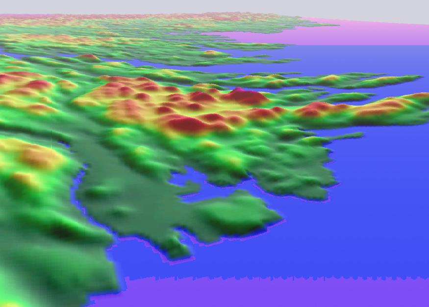
Figure 6 Perspective View of Colour Shaded Relief.
In addition to the perspective view a FLY was also generated over the digitally rendered colour shaded relief of
the Makkovik province. This option was made available to us through the PCI software and provided another
means of viewing the topographic data. The FLY feature saves a series of snapshot perspective views that will
be played in series as a short movie clip of the flight path over the image scene. This FLY movie can only be
viewed with a PCI FLY viewer.
To overcome the software limitations of the FLY we have converted the FLY movie loop file into a mpeg file.
The mpeg file type is a much more common animation file extension and can be read by most viewing devices.
A copy of one such movie players will be included with the data so our sample FLY can be viewed.
(This particular MPEG player is called "HYMPEG", and our FLY MPEG movie loop is called Short.mpg)
Regional Study (Labrador)
Throughout the project a second series of images were also generated on a smaller scale for the whole of Labrador.
The very same techniques and principles were applied to generate these images. The smaller scale
of the scene increased the size of the pixels to 800m to be at similar pixel dimensions as the other input data
sets. All of the input information was resampled with a bilinear transformation to a value of 800m, so that
it can properly displayed. The products from this investigation are included on a second plot of the data that
accompanies the Makkovik plots.
On one particular full Labrador plot we were able to produce a chromadepth colour shaded relief product that
included bathymetry for the continental shelf off of the coast. Other plots that were prepared for the whole of
Labrador included geophysical data like the 800m resolution Total Field Magnetics and the 800m Bougeur Gravity.
These geophysical layers were also plotted out in a hard copy form using the ACE plotting software provided
through PCI.
Through the presentation of the geological and topographical data for the whole of Labrador we were better able
to interpret how the Makkovik province fits into the regional Canadian Shield geology. Through the usage
of our whole Labrador scene one can easily be impressed by the geological diversity present in Labrador. This
range in lithology and structural history can better be understood and interpreted with more realistic spatial
displays of the data.
Conclusions:
The results that have been generated throughout our data integration and display have provided us with some new
and interesting means of visualizing the surficial geology and topography of the Makkovik province. The larger
scaled study of the area just including the Makkovik contains many interesting geological landforms that are made
apparent through the use of our DEM. The relief that is provided by the DEM provides the realistic topography
in our 3D imagery. The relief, combined with vectorized geological contact data tends to overlay the geophysical
data closely, corresponding to unconformity or structural features. It is this very nature of the combination of the
DEM with derived geological interpretations that provides alternative means of interpreting results of Lithoprobe
transect results. The interpretations of these transects can therefore be aided with the assistance of more realistic
composite displays of surficial geology.
For interest�s sake several interesting examples of relationships between thematic data and the DEM have been chosen
and displayed. These geological features are some of the more obvious examples of the relationship between the DEM
and the geology.
Figure 7 Notice the batholith or circular intrusion at the centre of the colour shaded relief image.(cross hair is on the feature)
Figure 8 This Total Field Magnetics Image has the same intrusion in the centre of this image, as demonstrated by the circular region of high returns. (two separate 400m magnetics panels are displayed in this image)
Figure 9 This colour shaded relief image contains evidence of faulting and fractures of the country rock, as displayed by the various lineaments and sharp edges detected in the DEM.
Figure 10 This image contains the linearly enhanced chromadepth colour-shaded relief >with the known contacts (blue) and faults (black) overlaid on top as vectors. The large fault in the top left of the image stops abruptly but may extend along the deep valley off of the edge of this image.
Figure 11 The Makkovik study area displayed as a chromadepth colour shaded relief image. Note the lineaments that are evident in the image, and the Makkovik province which appears as a wedge shape in the centre of the image.
Figure 13 The Total Field Magnetics for the entire Makkovik study region.
This project also included a poster and a 40 minute presentation of the data sets and findings that was presented at the Bedford Institute of Oceanography (BIO), in Dartmouth Nova Scotia.